Seven

After my post on five-fold symmetry, I can hardly keep myself from writing about seven. It seems unlikely, but the number seven does have some surprising properties, which I will illustrate. For instance, despite being called an octave, the diatonic musical scale really consists of seven notes: C, D, E, F, G, A, and B. With a remarkable sense of synesthesia, some people like to think each note has a color to it. I have folded my concept of the colors of notes into a paper aperture for your amusement.

Musicians like Alexander Scriabin developed systems to assign colors to key signatures based on the circle of fifths. The famous Hungarian composer and piano virtuoso, Franz Liszt, had a famous quarrel with Russian composer Nikolai Rimsky-Korsakov about the colors of the various key signatures; they saw them quite differently.

Seven is an odd prime number. Because it divides evenly into 1001 (and 1001*999 is one less than one million) its reciprocal has a six-digit repeat block, and thus seven the first number to have a repeat block that has length equal to the number minus one. It is a noble prime.

999999 = 3*3*3*7*11*13*37

Note that 7 and 13 have six-digit reciprocals, but 7 is often associated with good luck and 13 is often associated with bad luck.

An odd, prime number like 7 would seem to be impossibly irregular until you try to lay out seven pennies upon the table, as I did when I was five or so. I was surprised that it made the most elegant, regular arrangement possible.

And the seven pennies introduced young me to hexagonal packing. You can see that seven hexagons can make a hexagonal cluster. This is because it is a hexagonal number. The numbers 1, 7, 19, 37, ... , expressed as

1 + 6*T(n)

(where T(n) is the nth triangular number), are called hexagonal numbers because they give the exact number of smaller hexagons that can be put together to form a larger hexagon.

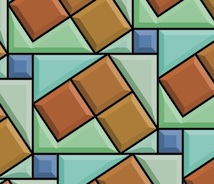
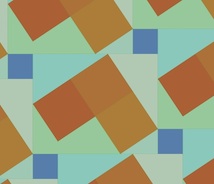
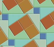
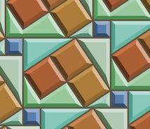
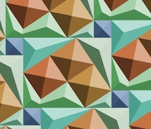
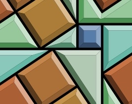
The clusters themselves can be fitted together. into an elegant offset packing, here shown using my Tile Patterns application. And a little help from Painter.

When I constructed this tiling, I had to work it out by hand first before I could enter it properly into Tile Patterns.

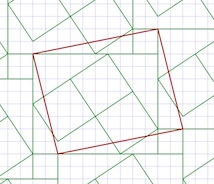
Here is my sketch of this tiling, giving some indication of the way I wanted to see it. Perhaps if we had hexagonally-packed eyes like the honeybee, and saw everything in these patterns, we would make our homes like they make their honeycombs.

It is only because my eyes are not hexagonally packed, I know, that I couldn't quite get the proportions right.

The green dashed parallelogram shows the repeat block of the offset tile pattern. It is because I like to think in squares and cubes that I can see it.

Seven is an interesting number for cubes as well, because it is one less than the cube of two.

Here I have illustrated that concept for you. It's always easier to see it visually than to just read it, I think.

Put one cube in the missing corner and you can make a 2x2x2 block. Two cubed is eight. So this shows seven cubes. Plus, I like a good graphic!

When it comes to seven, we do spend a bit of time dancing around six and eight.

The first diagram I showed was a folded paper aperture with seven sides. Its outline is a seven-sided regular polygon, called a heptagon.

Connect the corners of a heptagon and you can make various forms of seven-pointed stars.

Many countries use five-, six-, seven-, and eight-pointed stars as their symbols. Normally there are the wide star and the thin star. The Sheriff's Badge symbol uses a seven-pointed star that's somewhere in-between the two.

Other than these I don't really know other ways that the seven-pointed star gets used. This illustration I have created is a mandala form. I have applied a little color so you can see the various shapes better.

Seven dots on a grid can be situated in several different ways. But if you look at seven as two times four minus one, then you can see how a corner of one square may be shared with the corner of another square.

Each number is unique and interesting. In music, there is more to seven than just the diatonic scale. There is also music that features seven beats per measure, like Money by Pink Floyd, Solsbury Hill by Peter Gabriel, and the final Precipitato from Prokofiev's Piano Sonata No. 7 in B-flat. When I get in a mood, I will use this time signature. Usually it is broken up into two-two-three.

Finally, did you know that graph theory is based upon Leonhard Euler's solution to the problem of the Seven Bridges of Königsberg? Walk through the city, crossing each of the seven bridges exactly once. Once again the number seven provokes thought. Euler abstracted the two sides of the river and the two islands into four nodes and the bridges were thus abstracted into the seven arcs between them. The number of arcs attached to each node is called the degree of the node. If a node has even degree, then any path can enter and leave the node in an equal pairing. But if a node has an odd degree, then either the path must start or end there. It is easy to see that if more then two nodes have odd degree it is impossible for a single path to traverse all nodes, using the arcs between them. This is because a path must have only two endpoints. Königsberg's graph has four nodes of odd degree. Thus no such walk can exist.

So the number seven was actually the doorway to graph theory in the eighteenth century!

Patterns, Part 7

The Tile Pattern Designer is coming along. In it, you design a tile pattern in a parallelogram repeat block. This gives you quite a bit of leeway, with the ability to design triangular and hexagonal tiles, as shown in Patterns, Part 5. Using a grid to design tile patterns in this way is sufficient to plot out most of the tile patterns from the floor of the San Marco Basilica in Venice, as shown in Patterns, Part 6.

Now I will show you some of its features, all based on complex analytic geometry, which you can learn about in How Does It Work, Part 2.

First I design a pattern by drawing lines between grid points. This one took only eight lines, using a slightly rotated rectangle as the basis. I am careful to leave a few unusual shapes for open areas. This is so I can show you how the beveling works later.

I base it on a staggered block pattern, but I also place some rotated rectangles inside the largest rectangle.

I suppose I could have been a little more fancy in my design, but I wanted to show a few of the characteristics that you can control to render your tile patterns. The first, which you are familiar with, is the automatic recognition of closed polygonal areas.

Here I show the polygon areas.

The pattern is really made up of line segments that are automatically divided up. Then they are arranged into a graph, with nodes at the places where the segment ends meet. Then I mark each segment so both sides of it get visited. And start tracing counterclockwise to collect closed polygon areas. The complex part is how to handle holes and stand-alone polygons, but we'll talk about that some other time.

By the way, the graph is special because it wraps around just like the pattern does.

There is a tool to put color into each of the polygons directly. I have chosen an "earth and aqua" color scheme: surf and turf.

Next I bevel the edges of the polygons. This is actually complicated. It involves a gabling operation as we will see in a moment.

A bevel is shaded using an interesting model which predicts its color in HSV space based on the base color of the polygon and shading from the angle of the edge it is derived from. You can adjust the overall light angle in the interface.

The cool thing about polygonal display is that you only need to create the polygons once. Then you just need to evaluate all the copies on screen within the view. It's a bit messy to do that!

The bevel width is controllable, allowing you to magically adjust the look of the tiles directly with a slider. For me, it's a bit disorienting to change the bevel width, because I am not used to seeing this occur in real time in the real world.

I have made the computation of the bevel geometries bulletproof, a thing I was not able to accomplish at Fractal Design (and Metacreations) when I was trying to create the first version of this tool.

It appears that I've learned a few things since then! With previous posts, I have created the bevels by hand, by designing polygons on the grid. Now The bevels can be created automatically from the source polygons using a non-destructive procedural process. In other words, they can also be turned off if you like.

There is also a grout control. This means you can change the grout width in real time with a slider as well. This can make tiles that look a bit more real, since real tiles do have grout in between them.

The grout operation uses the beveling engine, so even if a tile disappears because the grout is so large, it knows not to output it.

And yes, it is disorienting to change the grout width in real time as well! When you move the slider fast, it's just crazy!

And, of course, you can turn the grout off if you like.

The beveling is completely general. If you crank up the beveling width until it is large enough, the center parts of the tiles disappear. This is why I call this a gabling operation.

The actual polygons output are really equivalent to the computations required by architects when they are producing gables for a roof of an oddly-shaped house.

I'm glad it works, because sometimes the polygon shapes are non-intuitive! It seems to be bulletproof now, and works in the general case. Like I said, I use this same engine for the grout computation as well.

One more problem presented itself when I was building this tool: the matte edge problem. When rendering polygons that abut each other, you get a tiny matte edge. I have made the background black to make this more obvious.

This problem occurs because I am using a standard polygon renderer (CoreGraphics bezierPath) and each polygon is output with anti-aliasing. This means that the edges will have a one-pixel-thick one-quarter-intensity dropout between them.

I remedy this by enlarging each polygon by 0.24 pixels before I render it. This can't really be done properly by stroking the edge (as in Postscript). It must be done by widening the polygon. So I built a widening engine into my tile engine.

All of the other diagrams show the result of this widening setting.

I think next I will do some work in refraction. With just a bit of work, it could look just like stained glass. This would require me to make the results actually 3D. Actually, that's not too hard, given the gabling model I use to compute the bevels.

Perhaps one tile could shade its neighbor. Or a global illumination model could give the rendering a bit more life.

Now, what does real marble look like?

Texture, Part 1

I am a bit of an expert on seamless tiling textures, since I created nearly all of the paper textures that ever shipped with Painter, Dabbler, Sketcher, and Detailer. But, how they were created?

This is the first post of many that actually resurrects the application, called Texture, which was used to create all the paper textures in Painter. This application hasn't run since 1996, and was forgotten until now. It was a secret application, that never saw the light of day outside the walls of Fractal Design and my house. But history is littered with lost arts. So now I will show you the art of making stuff that helps you to make art.

Speckles

It mixed tiling patterns with Fourier transforms with speckles. A speckle (or speckle pattern) is a set of points in the plane that repeats. But one where you almost can't see the tiles.

I show you one to the right, which has about 1.4 repeats of the tile in it. It does take some time to see the repeat, but it is there.

As opposed to the harsh repeat pattern of rectangular tiles, a speckle is visually pleasing and it is intended to be totally seamless.

It also seems like a very good start for creating paper textures because the texture has only one predominant spatial frequency. Now, a typical paper texture in Painter is 256x256 pixels, although they are scalable. This speckle has 1000 points in the tile, meaning that any derived paper texture will have about (256 x 256) / 1000 or about 65 pixels per item in the texture.

Creating a Speckle

First, the a tile is seeded with a number of random points. Lets say that you have constructed a function urand(), that returns a random floating point number on the range 0...1. Then the following code will suffice to create a random 1000-point speckle:

#define MAXSPECKLE 10000
int i, npoints = 1000;
point speckle[MAXSPECKLE];
for (i = 0; i < npoints; i++)
{
    speckle[i].x = urand();
    speckle[i].y = urand();
}

The random speckle is shown to the right. The dots are smaller because the average minimum distance is quite small, and we need to be able to see the individual dots.

Then we do an interesting trick. We iterate an anti-gravity transform to push the points apart in the plane. This uses a technique of mutual-avoidance to make them regularly spaced.

After about 10-12 iterations of the mutual-avoidance transform, this set of speckles looks like the one shown to the right. The spots are larger again because the average minimum distance has reached a steady state of about 6 to 8 pixels.

Tiling Math

On a wrap-around tile, certain things we take for granted like distance formulas become a bit different. For any two points p1 and p2, the distance can't be calculated in the normal way. We must account for the wrap-around.

To do that, we have to make a wrap-around rule that says if a point is more than one-half a tile forwards, then the image of that point behind us is really the one we want.

So, something like point-to-point distance becomes a bit more complicated:

float dist(point p1, point p2)
{
    float dx, dy;
    dx = p1.x - p2.x;
    if (dx > 0.5) dx -= 1.0; else if (dx < -0.5) dx += 1.0;
    dy = p1.y - p2.y;
    if (dy > 0.5) dy -= 1.0; else if (dy < -0.5) dy += 1.0;
    return sqrt(dx*dx + dy*dy);
}

The above function implements the wrap-around rule for a tile that repeats in both x and y.

To implement the mutual-avoidance iteration, we first make a pass over all the points in the speckle, looking for neighbors within a small distance. This optimum distance is usually computed in the following way:

effectRadius = 2.5 * sqrt(2 / (points * sqrt(3)));

This assumes that the tightest packing of points is a triangular packing. The 2.5 is thrown in as a fudge factor to make sure we get enough neighbors to do the right thing. Then we compute a motion vector for the point that is designed to push it away from its nearest neighbors. The following code shows this motion vector gathering pass. Note that, to right I have placed the initial state and the first six iterations of mutual avoidance, so you can see the effects of the iteration.

int i, j;
float d, mindist, avgmindist;
point *p1, *p2;
vector vs;
avgmindist = 0;
for (i = 0; i < npoints; i++)
{
    p1 = &speckle[i];
    vs = vector(0,0);
    mindist = 1;

    for (j = 0; j < npoints; j++)
    {
        if (j == i)
            continue;
        p2 = &speckle[j];
        d = dist(p1, p2);
        if (d > effectRadius)
            continue;
        if (d < mindist)
            min_d = d;
        vs += (*p1 - *p2) / (d*d);
    }

    p1->v = vs;
    p1->dv = length(vs);
    p1->mindist = mindist;
    avgmindist += mindist;
}
avgmindist /= npoints;

The above code also computes an average minimum distance, so we can properly scale the motion vectors for the points.

Next, we compute the sum over all motion vectors' velocities (lengths) and create a factor that helps us normalize the motion vectors.

float dvs, factor;

dvs = 0;
for (i = 0; i < npoints; i++)
{
    p1 = &speckle[i];
    dvs += p1->dv;
}
dvs /= npoints;
if (dvs == 0)
    factor = 1;
else
    factor = (effectRadius * 0.04) / dvs;

This factor can be used to scale the motion vectors to complete the avoidance iteration. The points are now moved. They must be placed back on the tile if they wander off, of course.

for (i = 0; i < npoints; i++)
{
    p1 = &speckle[i];
    p1 += factor * p1->v; // move the point

    if (p1->x < 0.0)
        p1->x += 1.0;

    else if (p1->x >= 1.0)
        p1->x -= 1.0;

    if (p1->y < 0.0)
        p1->y += 1.0;

    else if (p1->y >= 1.0)
        p1->y -= 1.0;
}

And that's how mutual avoidance works, in a nutshell.

The best thing about speckles is that they can also be used for so many other things. One of these is visually interesting, since it mimics the arrangement of cells in the back of your eye. For instance, to the right we can see a section of the human fovea, the dense cluster of photoreceptor cells in the back of your eye. It is interesting how often cells land in a hexagonal tight-packing.

One day, when implementing Texture, I came across a computation geometry trick called Voronoi maps. These are like a cellular partitioning of space around a set of points. Arranged so each point gets its own well-defined little capsule of space. This technique was very interesting visually.

Here you see a Voronoi map applied to a speckle. The speckle was created by starting with 100 random points and iterating the mutual avoidance iteration a mere 9 times.

Then a Voronoi map was created on the tiling plane. This is a bit trickier than constructing a Voronoi map in general, but really only the distance function needs to change.

I won't go into how I create them, but I will give a link to a remarkably efficient technique for creating them. Most techniques for creating these maps depend upon the simple in-circle test.

But there are other ways to treat points: connecting them. An example of this is called a tree of points.

Spanning Trees

A spanning tree is a single graph that connects all the points of the graph, but which does not contain a single loop. To construct one, maintain a tree number for each point. When you connect two points, set their tree numbers to the minimum of the two tree numbers of the two points. Do not connect them if they have the same tree number, since that would imply a loop.

So, the art in spanning trees can be put simply: in what order do we connect the points?

I call this the function type of the spanning tree.

This kind of function is used in constructing halftone dot patterns as well, but that's a post for another day!

Here we have one spanning tree, constructed so that the bonds are favored to fan out from the center.

This kind of tree is useful in producing growth-like looks. Really, it is more like the growth of bacteria or lichens, since it is constrained to lie in the plane.

Another kind of spanning tree is constructed on the same points, but in this case, it is designed so the bonds are favored in a direction perpendicular to those of the first spanning tree. This is useful in creating rose-petal patterns and even fingerprint patterns.

There are more things you can do with speckles, and bridging the gap between geometry and image processing is the key.

We will talk more about that in future Texture posts.

But, have no fear, I have taken step 1 in bringing the art of creating paper textures back from the dead!

Patterns, Part 2

Back in 1993, I tested a special capability that, unfortunately, has since disappeared. It allowed you to devise patterns that used a set of basis tiles, so that each tile could be chosen from this basis set. I call these tiling grammars.

At the right is an example of such a pattern. When I write pattern, I mean a non-repeating arrangement of items taken from a small set.

In this case, you can easily see how a space-filling curve can be generated from a small set. But what isn't really obvious is that this image is made by randomly placing square images into a grid.

Each grid element can have one of two images in it. With this image, I have taken care to create an image that (almost) doesn't have any obvious loops in it.

Well, OK, it does have one, in the lower left corner. But it doesn't have any circles in it. That, it turns out would be legal in this particular pattern grammar. Loops (and loops within loops within loops) would also be legal.

Here is the basis set for this particular image. It consists of two tiles as you can see. In each square, one tile connects the middle of the top edge with the middle of the right edge and also connects the middle of the left edge with the middle of the bottom edge. The other tile is either a mirror-symmetry of the first, or it is rotated 90 degrees from the first, whichever you like.

But wait, there are more options along these lines. For instance, I can create two more tiles that connect vertically and horizontally. In one tile, the horizontal crossing takes precedence, and in the other, the vertical crossing takes precedence. Now what would happen if we randomly expressed a tile from this basis?

Well, we can easily generate this test as well. Here, to the left, we see that suddenly, this image is starting to look like a subway map.

This grammar can generate interweavings of any kind. Weavings are made of warp (vertical threads) and weft (horizontal threads). Since one element is warp-over and another element is weft-over, we can represent all possible interweavings.

But what makes this interesting is that the threads can also turn.

You can represent knots as well, of course, since we include pass-under and pass-over elements.

Suddenly, this pattern has taken on more dimensions than before. Just 4 elements and so much richness of representation!

I thought on this, and realized that I could also include ends: threads that do not cross the tile, but rather end. I increased the basis by 4 more tiles. This time, the four diagonal sad-faces were added.

It is not obvious to me what this grammar will generate. But I think it's going to be interesting nonetheless! This seems to leading to noodles and other patterns made of threads that have ends. What will it look like?

Here is an example output randomly from this grammar. The most interesting part is that the complexity has definitely increased. Notice that the threads seem to look like bacteria in a culture mold. But regular, of course.

One obvious thing is that dots have appeared. And letters, like lower-case f and t.

You can identify each thread by itself, and where it goes.

And yes, a sad face has appeared in upper right.

After making this, it occurred to me that it would be possible to add 3 more elements to the basis. A tile containing 4 ends, and horizontal and vertical crossings with ends on the other sides of the tile.

Here is the new basis set, with the three new tiles added.

Perhaps the new elements look like the division symbol. But with the interconnections, this will likely be obscured by the neighboring elements, hiding it.

One thing we can say just by looking at the basis set: there might be more dots than in the last generated example. And more vertical and horizontal lines, particularly those which have no other line crossing them. So this will undoubtedly lead to more open space in some areas.

Here is the result of generating a random placement using this new basis set.

The result is using fewer and fewer curves. There are twice as many free-floating dots as in the last one.

One thing to remember is that each previous level is really just a subset of this next level.

Perhaps even more interesting than ends is the possibility of branching. We can assume that there are no curves and try to construct a maze grammar.

This would not have crossings, per se, rather it would be more square, with cross, the four t's, horizontal and vertical paths, with ends as well, but not really circular or curved. It occurs to me to try this case.

Here is the new basis, that operates only horizontally and vertically, and contains branching. I don't think it could generate a maze, though. On the average, it will probably generate circuits (closed loops).

This grammar is very foursquare. I have rounded off the edges to make it a little more presentable.

Here is the result of generating a random placement from this basis set.

It is a very busy pattern with very few dots. It does tend to be a little maze-like, and the pieces in it are heavily connected.

The tiling grammars I have presented here are reminiscent of Wang tilings.

Perhaps they are even closer to Thue-Morse tilings.

All of these are related to the work I did back in 1993, when the image hose was just invented and I realized that it might bear on this class of tiling grammars.